Adapting to Cross-Domain Data in Object Detection: OMNIA Faster R-CNN
This is a brief review of the paper titled “OMNIA Faster R-CNN: Detection in the wild through dataset merging and soft distillation”. This is a fairly recent paper and solves a problem which is quite commonplace with object etectors.
Introduction
Widely popular object detectors like Faster R-CNN or SSDs depend on Full Supervision and need instance annotations for each object in each image. What would happen, if say, a new category of objects are introduced in the dataset, or one uses a dataset from another domain to test this trained model’s performance? These models are no virtuosos. Quite expectedly, they will perform really bad. This method aims to use several datasets with different categories to increase the number of categories that can be detected. It also uses concepts of transfer learning to enhance domain independence.
One simple approach to this problem would be to train highly specific models for such specific datasets. So, if one needs to detect instances in images pertaining to Fashion elements, one can train a model on very specific images that have instances belonging to categories that need to be detected. If someone needs to detect only cars, train a model on the Cityscape dataset. These models become real experts in their domain but will perform really poorly when tested on the other. We need models that can adapt to domains. In that regard, we would like to benefit from the training done on a more general dataset like MSCOCO and use that knowledge on a dataset like Cityscapes. That helps because it helps reduce false positives. Being able to detect bottles or fire hydrants improves prediction scores on cars by reducing False Positives.
Another approach could be to concatenate the two datasets and train a single model on it. However, the categories in both datasets might have zero or minimal overlap. Let’s say Category \(C_a\) is not present in \(Dataset_2\) and category \(C_b\) is not present in \(Dataset_1\). In that case upon training a single model on both datasets, all instances of \(C_b\) will be treated as background in all images of \(Dataset_1\) and all instances of \(C_a\) will be treated as background in all images of \(Dataset_2\). Thus, a full relabelling is needed.
Considering these problems, the principal contributions of this paper are as follows:
- A framework for dataset merging to train detectors that are robust on all categories from all merged datasets
- Detection without Forgetting because we train on several datasets simultaneously without any additional labeling.
- Alleviate missing annotations with model predictions as weak supervision, using ideas from self-training.
Before one reads this summary, it is expected of them to understand the full framework in Faster R-CNN and Fast R-CNN.
Approach
Notations
Two datasets \(D_a\) and \(D_b\) are being used. Dataset \(D_a\) is defined by categories \(C_a\) and images \(I_a\), with Ground truths \(G_a\). Similarly \(D_b\) has \(I_a\), \(G_b\) and \(C_b\).
Initial Training
Two Domain Adapted Faster R-CNN detectors are trained. The first detector \(Detect_a\) learns to detect \(C_a\) on \(I_a\), and has access to \(I_b\), without seeing the corresponding ground truth \(G_b\). The second Faster R-CNN is also trained accordingly. The aim is to make \(Detect_a\) as accurate as possible on \(I_b\) and \(Detect_b\) on \(I_a\).
Merging Procedure
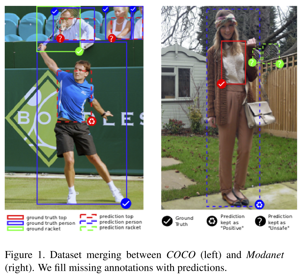
Self-Training: The principal aim is to train a detector simultaneously for all categories \(C_a U C_b\) on all images \(I_a U I_b\). The predictions of \(Detect_a\) on \(I_b\) serve as targets along with the existing Ground Truths \(G_b\). Likewise we get additional targets on \(Dataset_a\) along with \(G_a\).
Prediction Selection: One has to judiciously choose these cross-predictions based on the confidence score of prediciton. By setting two thresholds, one can classify the predictions as safe, unsafe, or discardable.
Model Framework
Region Proposal Network: Instead of assigning a binary label for foreground/background classification, like in Faster R-CNN, this method adds another undefined label to detect all proposals with an unsafe prediction.
SoftSig Box Classifier: The idea is to avoid the problem that we discussed earlier. Region Proposals from \(Detect_b)// on \(I_a)// will indeed serve as additional labellings but one cannot be completely sure that the predicted class is true. However, one can at least say that the predicted RoI is not a background. The custom loss function defined here takes care of these constraints. The loss is called SoftSig because it combines both SOFTmax and SIGmoid activation functions. The overall loss is:
\[L_{softsig} = L_{categorical} + \lambda_{binrary}L_{binary}\]
We discuss both components here, with the assumption that from a sample of \(R\) RoIs, we have a region \(r\) and it matches with a box of category \(c\)
1. Masked Categorical Cross-Entropy
This loss term is responsible for aligning predicted probabilities with targets and has a mask that helps discard this term for unsafe predictions.
\[ L_{categorical} = -\frac{1}{R} \sum_{r} \sum_{c} t_r^c log(softmax(x_r^c)) \]
Therefore, there is no loss backpropagation component from this categorical loss term for all unsafe region predictions. Since, we aren’t definitely sure about its classification, we cannot let it align with any given class in the ground truth. The mask \(m_r\) = 0 when \(r\) is an unsafe prediction.
2. Masked Binary Cross Entropy
Binary cross entropy treats the different categories as independent binary classification tasks. Each logit decides whether the sample belongs to a particular category \(c\) or not. A mask is applied to the predictions for all regions marked as unsafe predictions.
\[ L_{binary} = - \frac{1}{R(C+1)} \sum_{r,c} w_r^c (t_r^c log(sigmoid(x_r^c)) + (1-t_r^c) log(1-sigmoid(x_r^c))) \]
Thus, if a RoI matches with an unsafe prediction of category c, logits for background and that category will not contribute to the loss, while logits for all other categories will be decreased after an optimization step.
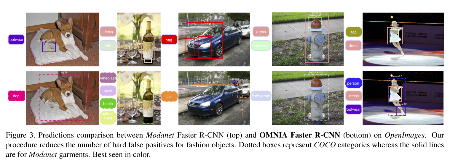
Results